An Introduction to the Minimum Description Length Principle
/
This is part 1 of a blog post on our ICML 2024 paper. In general I find the Minimum Description Length (MDL) Principle a super interesting way to think about learning, and think it’s a relatively underexplored direction within the community. This is my attempt to give a basic overview of the Minimum Description Length (MDL) Principle and the predictive Normalized Maximum Likelihood (pNML) distribution, which are necessary to understand part 2 which discusses our actual method itself. I’d recommend reading this one first unless you’re already familiar with MDL.
Given some data and a set of models that explain the data, how should we decide which model is best? If we simply choose the model that best fits our given data, we risk overfitting, but if we instead try to choose the simplest model, we risk underfitting. A good model selection principle needs to find a balance between these two extremes.
The Minimum Description Length (MDL) Principle does exactly this. In short, the MDL Principle is a version of Occam’s Razor that states we should select the model that best encodes the data. But what exactly does this mean? I’ll provide a simple example to give some intuition. $ \def\X{\mathbf{X}} \def\Y{\mathbf{Y}} \def\rY{\mathcal{Y}} \def\loss{\mathcal{L}} \def\cost{\mathcal{J}} \def\hparam{\hat{\theta}} \def\oparam{\theta^{\star}} $
On Codes and Codelengths
Suppose Alice and Bob both have some dataset $\X = \lbrace x_i \rbrace_{i=1}^n$ for which they’d like to know the labels $\Y = \lbrace y_{i} \rbrace_{i=1}^n$. Let’s assume $\X$ is a set of MNIST images, and $\Y$ are their corresponding labels 0-9. Let’s define $k$ as the size of the discrete label space $\rY$. Luckily Bob has access to $\Y$, so all he has to do is send the data over to Alice. Since he uses Comcast and they just raised their rates, he’d like to send it using the fewest number of bits possible.
First, we need to define a code, or a procedure for encoding a given $y_i \in \Y$, turning it into a series of bits.
Since Bob is only able to send an uninterrupted series of bits, this code also needs to be a prefix code, meaning no code is a prefix of any other code.
Let’s start by considering the simplest possible code, which we’ll call the Uniform Code $U$.
This code simply turns the label $y_i$ into its binary representation (e.g. 3 → 0011, 9 → 1001, etc.).
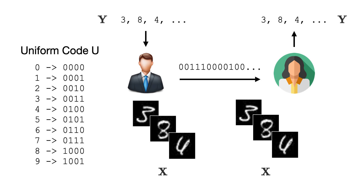 The Uniform Code $U$ assigns a fixed length binary encoding to each label
We’ll define a codelength function $\loss_U(x_i, y_i)$ which returns the codelength of $y_i$ given $x_i$ using the coding scheme $U$. Then the average number of bits to encode each example is \[ \cost_{U}(\X, \Y) = \frac{1}{n}\sum_{i=1}^n \loss_{U}(x_i, y_i) = \log k \approx 4 \] Since we’re measuring information in bits, whenever I use $\log$ I really mean $\log_2$.
Sidenote on Coding Precision
In our MNIST example Bob would be able to use only $\log 10 = 3.32$ bits per example in an alternate universe with fractional bits. In the real world of course this isn’t possible, and we have to round up to 4. However, for the purposes of this discussion and MDL in general, we can ignore these nuances about coding precision since they add up to a small constant.
Two-Part Codes
Of course this code isn’t perfect.
Since Bob and Alice both have access to $\X$, he knows that for a given $x_i$, certain labels $y_i \in \Y$ are more or less likely.
For example, if $x_i$ contains curved lines, we know it has to be a 0, 2, 3, 5, 6, 8, or 9, and if it doesn’t then we know it has to be a 1, 4, or 7 (obviously this depends on handwriting but let’s assume everyone writes nicely).
Can we use this to design a better code?
Let’s assume Bob has built a “curved line detector” $f_{\theta}$ with some parameters $\theta$, such that $f_{\theta}(x) = 1$ if the image $x$ contains curved lines. Now we’ll define a new code we call Curve Code $C$. To encode a given $x_i$, we first determine whether $f_{\theta}(x_i)$ is 1 or 0. Then we can use our original code $U$ but now with a reduced set of potential labels to encode.
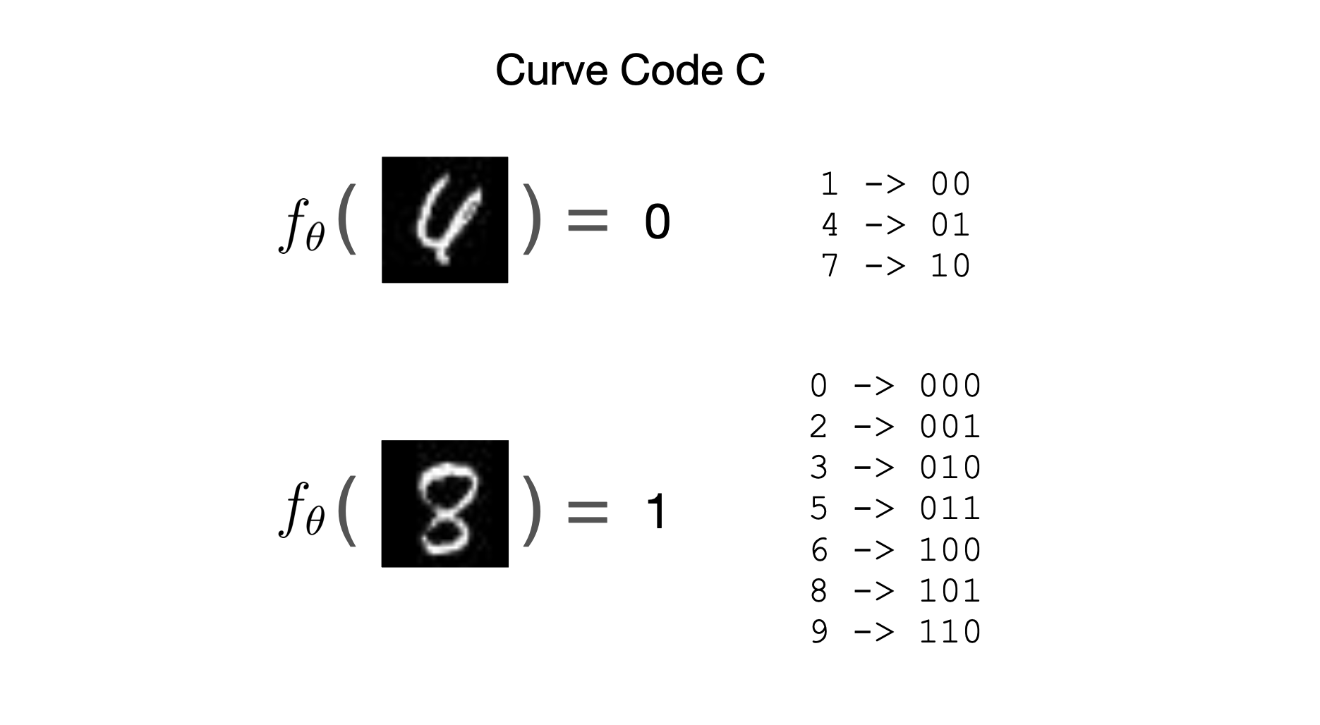 The Curve Code $C$ uses the output of the curve detector $f_{\theta}$ to choose a shorter fixed length code.
Our codelength function is then: \[ \loss_{C}(x_i, y_i) = \begin{cases} \log 3 \approx 2 &\text{if } f_{\theta}(x_i) = 0 \cr \log 7 \approx 3 &\text{if } f_{\theta}(x_i) = 1 \end{cases} \]
If we assume that the labels in $\Y$ have a uniform distribution among all possible labels, then with this new code Bob needs only \[ \cost_{C}(\X, \Y) = 0.7 \cdot 3 + 0.3 \cdot 2 = 2.7 \] bits per example to transmit all of $\Y$ to Alice! This reduces our average bits per example by 33% compared to our original code $U$.
Unfortunately we’ve left out a crucial detail here, which is that Bob also needs to transmit the parameters $\theta$ to Alice. To minimize the total codelength, we then simply need to pick the model with the fewest parameters $\theta$ that can still perform curve detection perfectly. We call a code that depends on first transmitting a model, then the labels encoded using a scheme dependent on the model, a two-part code.
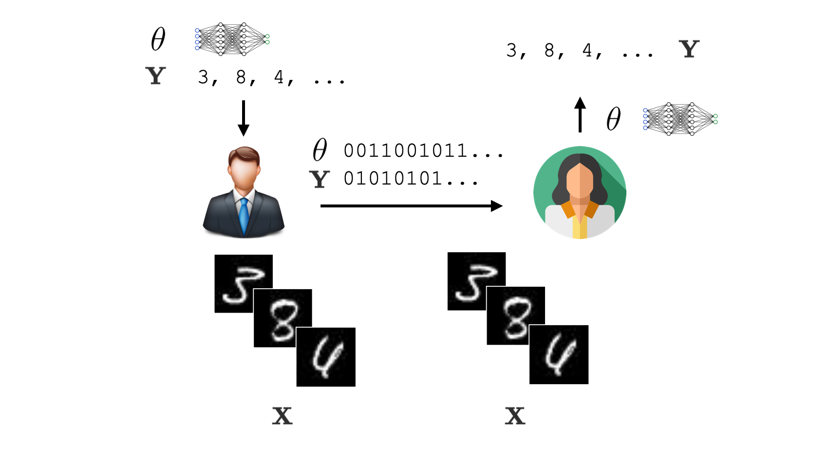 To transmit the two-part code to Alice, Bob first sends $\theta$, then sends the data encoded using one of the two codes depending on the output of $f_{\theta}$. To decode the data, Alice builds the model using $\theta$ then chooses the corresponding code based on $f_{\theta}(x_i)$
Learning as Data Compression
Still, our code can be improved. A curved line detector model is a great start, but what about adding a loop detector? Or a stroke detector? Perhaps what we really want is a model that gives us a code, such that, with high probability, we can transmit the true label with very few bits. To build this code, the Kraft Inequality tells us that we can always draw a one-to-one correspondence between a prefix code and a non-defective probability distribution $p$ over a finite or countable set $\mathcal{Z}$ of items that we would like to encode, such that the codelength for an item $z \in \mathcal{Z}$ is \[ \loss(z) = -\log p(z) \]
In other words, a good code corresponds to a model that produces a distribution that assigns high probability to the true label, and vice versa. This means that the more that we are able to compress the data, then the more that we have learned about the data (where learning here equates to finding regularities in data). This is the key insight of the MDL Principle, that learning is the same as data compression.
More concretely, lets presume we have some model $p_{\theta}(y | x)$ parameterized by $\theta \in \Theta$ that produces an output distribution over the labels given an example $x$. Let’s call the code that this distribution defines the Kraft Code $K$.
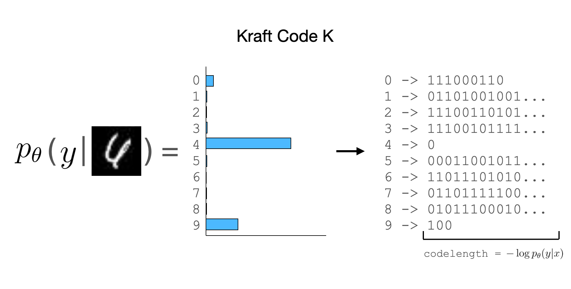 To decode the Kraft Code $K$, Alice builds the model using the parameters $\theta$, then decodes the bits using the code defined from the distribution $p_{\theta}(y_i | x_i)$. The codelength for each label is $-\log p_{\theta}(y_i | x_i)$
Notice that the higher the probability, the shorter the codelength, and the lower the probability, the longer the codelength. The average codelength per example is \[ \cost_{K}(\X, \Y) = \frac{1}{n} \sum_{i=1}^n \loss_{\theta}(x_i, y_i) = \frac{1}{n} \sum_{i=1}^n -\log p_{\theta}(y_i | x_i) \] If our model is parametric, then we incur a constant cost $|\theta|$ to transmit the model to Alice, and minimizing the codelength reduces to finding a set of parameters $\hparam$ that minimizes $\cost_{K}(\X, \Y)$ well. The model $\hparam$ will then have successfully compressed and learned the data.
Since the codelength corresponds to the log loss, the objective above should look very familiar as the standard maximum likelihood estimation (MLE) objective. In other words, for parametric model classes, MDL reduces to MLE. However, unlike MLE, MDL does not make any assumptions about the data being sampled from some distribution, and indeed does not assume any notion of ground truth at all. All MDL is concerned about is compressing the data well.
Regret
Once Bob has successfully trasmitted all of $\theta$ and $\Y$ to Alice, suppose they both recieve a new unseen data point $x’$ for which they’d like to know the corresponding label $y’$. Since they both have access to the base model $\hparam$ trained on the original data, Bob can transmit the label using the base codelength $-\log p_{\hparam}(y’ | x’)$.
However, since Bob only minimized the codelength on the original dataset $(\X, \Y)$, his code for $x’$ may not be great. Let’s suppose Henry is given the same task as Bob to transmit the labels $\Y$ and $y’$ to Alice, but gets to learn his model and code using all of the data. Then instead of minimizing the codelength on only the original dataset, he can instead find the parameters $\oparam$ that minimize it on an augmented dataset that also contains $(x’, y’)$: \[ \oparam(x’, y’) = \arg\min_{\theta \in \Theta} \cost_{\theta}(\X, \Y) - \log p_{\theta}(y’ | x’) \] We call Henry’s model the hindsight-optimal model since it’s the model that Bob would have used in hindsight if he had known that he needed to encode $(x’, y’)$ as well. The codelength $-\log p_{\oparam(x’, y’)}(y’ | x’)$ is called the hindsight-optimal codelength.
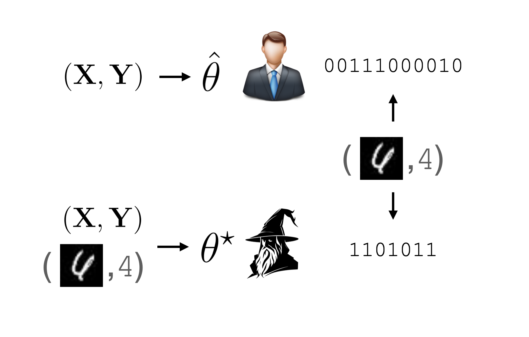 Henry (shown as the wizard here) is allowed to cheat and observe the test point he needs to encode while Bob cannot.This means he can build a better code and transmit the data to Alice using fewer bits.
After both transmitting their data to Alice, Bob and Henry meet up and compare codes. Bob experiences a regret: \[ R(x’, y’) = -\log p_{\hparam}(y’ | x’) + \log p_{\oparam(x’, y’)}(y’ | x’) \] that corresponds to the number of extra bits he had to use to transmit the data. If $x’$ was also an MNIST image, then Bob might not feel too bad, since his code should perform quite well already. However, if $x’$ is sampled from another dataset or distribution entirely, then Bob’s model might have performed much worse compared to Henry’s.
Sidenote on Predictive Coding
Traditionally in the MDL literature we would care about the entire codelength for transmitting both $\Y$ and $y’$, and not just $y’$ (since ultimately we want to use MDL for selecting a model that learns over all of $\Y$ and not just $y’$). This only slightly changes all of the math in this post (simply replace every sum over $y \in \rY$ with a sum over all possible sets $\lbrace Y, y \rbrace \in \rY^{n+1}$). I’ve opted here for the predictive coding setting since this makes understanding the ideas a bit easier.
The Predictive Normalized Maximum Likelihood Distribution
Bob goes home and vows to design a code that does almost as well as Henry’s on $(x’, y’)$, up to some constant amount. We call such codes universal codes. The code Bob comes up with is the predictive Normalized Maximum Likelihood (pNML) distribution, which ensures that no matter what $(x’, y’)$ are given to him, he’ll feel as little regret as possible. It is defined as follows: \[ p_{\text{pNML}}(y’ | x’) = \frac{p_{\oparam(x’, y’)}(y’ | x’)}{\sum_{y \in \rY} p_{\oparam(x’, y)}(y | x’)} \] Intuitively, pNML attempts to assign to each label the maximum likelihood probability, then renormalizes to achieve a valid probability distribution (hence normalized maximum likelihood).
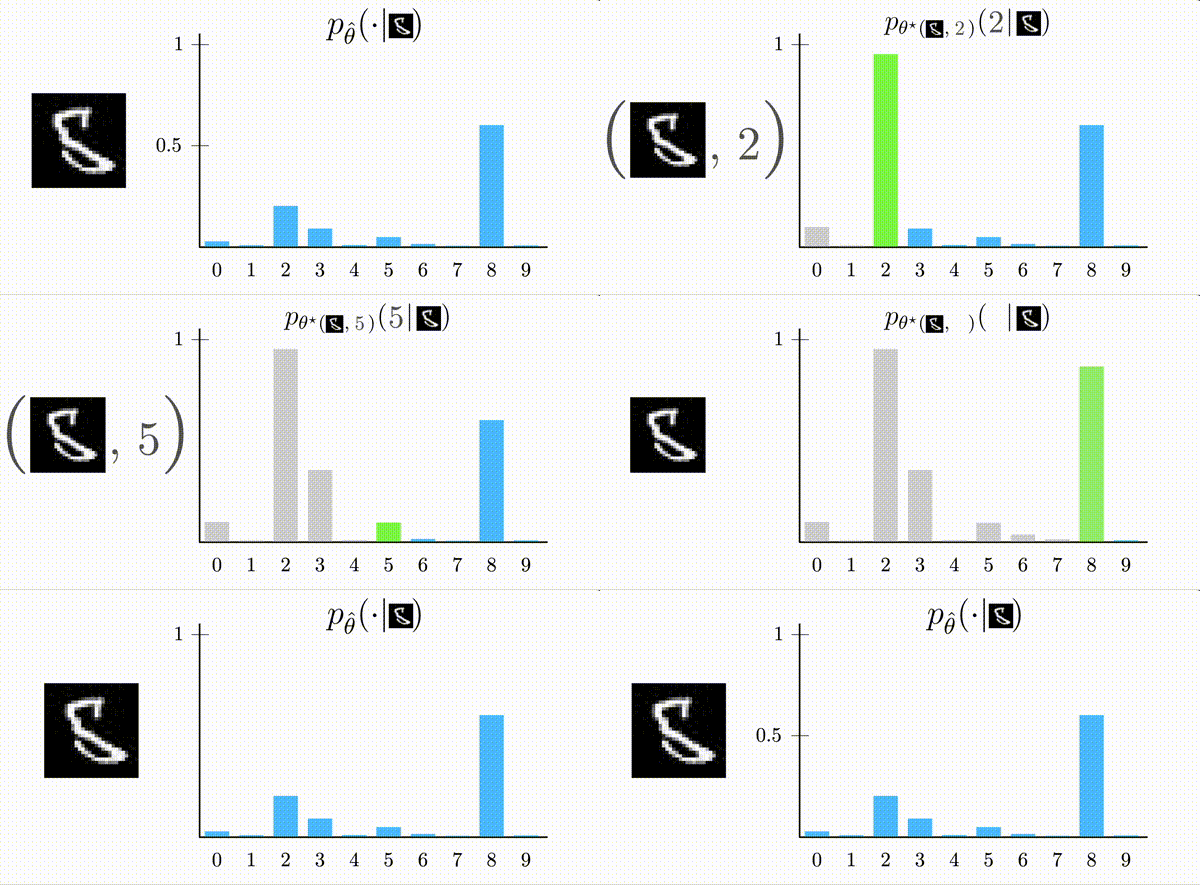 The pNML distribution tries to assign the hindsight-optimal probability to each label, then renormalizes by their sum to produce a valid output distribution. In this example the pNML distribution accurately reflects the model’s uncertainty between the
 2 and 8 labels
If Bob uses the pNML code, no matter what label $y’$ is assigned to $x’$, Bob experiences the same regret: \[ \begin{aligned} R_{\text{pNML}}(x’, y’) &= -\log p_{\text{pNML}}(y’ | x’) + \log p_{\oparam(x’, y’)}(y’ | x’) \cr &= \left( -\log p_{\oparam(x’, y’)}(y’ | x’) + \log \sum_{y \in \rY} p_{\oparam(x’, y)}(y | x’) \right) + \log p_{\oparam(x’, y’)}(y’ | x’) \cr &= \log \sum_{y \in \rY} p_{\oparam(x’, y)}(y | x’) \cr &= \text{COMP}(\Theta, x’). \end{aligned} \] Since any distribution $p \neq p_{\text{pNML}}$ must have some label $y$ that it assigns lower probability to compared to the pNML distribution, the worst case regret for $y$ must be larger for $p$ than for pNML, so pNML is minimax optimal.
This regret is also called the parametric complexity (COMP) of $x’$ relative to the model class $\Theta$. COMP is independent of the true label $y’$, and measures the number of essentially different distributions within $\Theta$ that fit $x’$. A larger COMP means the model class $\Theta$ is more expressive for modeling the data $x’$.
The codelength of the pNML distribution is also called the stochastic complexity of $(x’, y’)$ relative to the model class $\Theta$: \[ \begin{aligned} \Gamma(x’, y’) &= -\log p_{\oparam(x’, y’)}(y’ | x’) + \log \sum_{y \in \rY} p_{\oparam(x’, y)}(y | x’) \cr &= -\log p_{\oparam(x’, y’)}(y’ | x’) + \text{COMP}(\Theta, x’) \end{aligned}\] where the first term is the hindsight-optiomal error, which is the amount of error we can expect from our model even when observing the true label. The second term is the parametric complexity as above.
The stochastic complexity measures something like the amount of “essential information” contained within $(x’, y’)$ relative to the entire model class $\Theta$ (and original training set $(\X, \Y)$). In order to minimize this codelength, we need to ensure that our model is expressive enough to achieve a low hindsight-optimal error (avoiding underfitting) while avoiding an overexpressive model with high parametric complexity (avoiding overfitting). Using pNML and its associated code to perform model selection thus achieves the balance we hoped to find.
Beyond Model Selection
If you’ve made it all the way to the end, you might be asking why we should care about pNML and stochastic complexity outside of selecting a good model. In general, the framing of learning as compression means we can quantify certain vague notions of complexity and uncertainty by couching them in concrete terms of codelength and regret with specific interpretations in information theory. Here are a few ways these equivalences can be useful:
-
Uncertainty Calibration: Since the pNML distribution is minimax optimal with respect to the regret, it captures an inherent notion of uncertainty about the model’s prediction and should be better calibrated when making predictions. Intuitively, if our model can fit any arbitrary label to the data, then its prediction is highly uncertain. If a particular choice of label is much easier to fit than the others, then its prediction has low uncertainty.
-
Mislabel Detection: If an example $x_i$ has been assigned an incorrect label $y_i’$ when it should have been assigned a label $y_i$, simply examining the model error is not enough since modern neural networks can easily overfit any arbitrary data. Luckily, these examples should have a much higher stochastic complexity, since the hindsight-optimal model can fit $x_i$ much better using the correct label $y_i’$ instead of the incorrect label $y_i$. Correctly labelled examples should have lower stochastic complexity, since only one labelling (the correct one) should be consistent with the rest of the data.
-
OOD Detection: If our model observes an $x’$ at test time that is substantially different than the original training set, then it should contain a lot of information relative to the model class, regardless of its label. Since we don’t have access to $y’$ (and may also have no guarantees any reasonable $y’$ can be defined), we can simply measure the parametric complexity as a way of comparing how “similar” this example is to the training set. This comparison should allow us to detect out-of-distribution (or from an MDL perspective, outlier) examples well.
Unfortunately, calculating the pNML distribution and stochastic complexity in practice can be difficult or even impossible. Consider that for just a single example $x’$, we would need to optimize $k$ separate hindsight-optimal models for every possible labeling $y’ \in \rY$. Even if we do so, we may find out that our model is so expressive it can fit all arbitrary labellings perfectly well. How then can we practically use MDL for any of these tasks? Check out part 2 to find out!