hi, i'm nathan ng

This is part 2 of a blog post on our ICML 2024 paper. This one goes into the method itself, while part 1 goes into the background on the Minimum Description Length Principle and normalized maximum likelihood. I’d recommend reading that one first before this one unless you’re already familiar with MDL.

---

$ \def\X{\mathbf{X}} \def\Y{\mathbf{Y}} \def\rY{\mathcal{Y}} \def\loss{\mathcal{L}} \def\cost{\mathcal{J}} \def\hparam{\hat{\theta}} \def\oparam{\theta^{\star}} \def\param{\theta} $ If you’ve been around the internet recently you might have seen posts showing Google’s Gemini saying some strange things:

Either I’m way behind on my daily rock intake or Gemini is making up information it knows nothing about. If we want to be able to use these LLM systems (and in general any kind of AI system) in real world settings, we’ll need better ways to tell when they’re actually confident in their predictions, and when they’re simply making things up.

A classical approach to this problem would use Bayesian principles to better quantify uncertainty, but these methods face significant scalability challenges. In our paper we instead choose to take a Minimum Description Length (MDL) Principle based approach to quantifying uncertainty.

Specifically, for a given query example $x$, we consider, for every possible label $y’ \in \rY$, asking the question “How well could my model class fit this additional training point $(x, y’)$ along with the original training data?” We call the model trained with this additional training point the hindsight-optimal model and the original model the base model. If any arbitrary label $y’ \in \rY$ could be fit by the hindsight-optimal model, then our prediction for $x$ should be highly uncertain. In contrast, if one label $y$ can be fit much easier than the others, then our prediction should have low uncertainty.

This notion is captured by the pNML distribution, which calculates the hindsight-optimal MLE for the original training data and the additional training point $(x, y’)$, then renormalizes across all labels: \[ p_{\text{pNML}}(y | x) = \frac{p_{\oparam(x, y)}(y | x)}{\sum_{y \in \rY} p_{\oparam(x, y)}(y | x)} \] where $\oparam(x, y)$ is the hindsight-optimal MLE for the additional point $(x, y)$. Intuitively, pNML attempts to assign to each label the maximum likelihood probability, then renormalizes to achieve a valid probability distribution (hence normalized maximum likelihood).

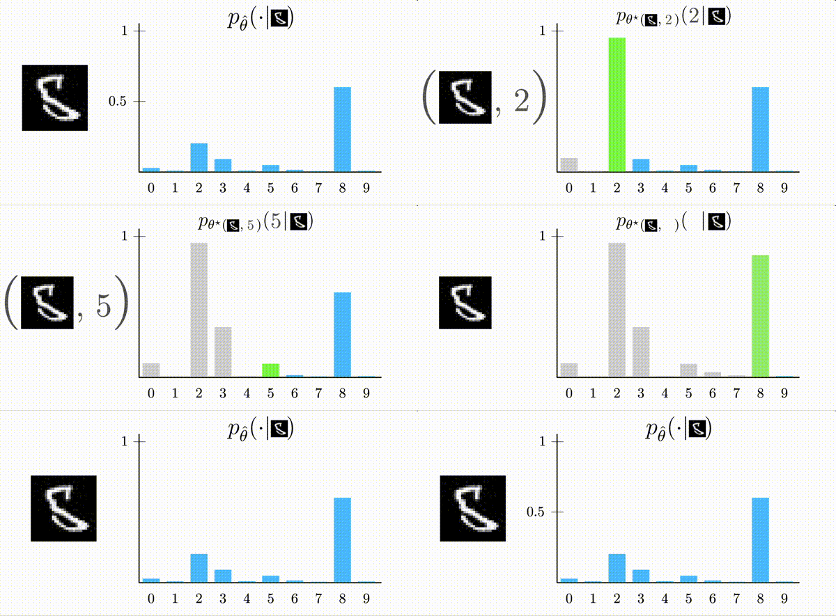The pNML distribution tries to assign the hindsight-optimal probability to each label, then renormalizes by their sum to produce a valid output distribution. In this example the pNML distribution accurately reflects the model’s uncertainty between the 2 and 8 labels

The negative log of this distribution, or its codelength, defines the stochastic complexity of $(x, y)$. This gives us a sense of how much “essential information” is contained within $(x, y)$ relative to the model class. Examples with high stochastic complexity may be more likely to be OOD, mislabeled, or simply difficult to learn.

Warning: there’s a bunch of math ahead and not a ton of pictures. If that doesn’t sound particularly interesting, read the TL;DR below then skip to the results:

TL;DR

Our ultimate goal is to estimate the output probability of the hindsight-optimal model for all possible labellings of a given input example. To efficiently and accurately estimate this value for deep overparameterized neural networks, we solve 3 key issues.

1. First, to prevent the model from memorizing the additional example, we use a proximal objective that penalizes movement in function and weight space away from the base model trained on the original data.
2. Second, to soften the function space proximal term, we apply temperature scaling to the model’s outputs
3. Third, to efficiently estimate the hindsight-optimal model output, we linearize the model about the base parameters, which corresponds to a temperature-scaled Boltzmann influence function.

Combining these together, we formulate a pNML code and corresponding complexity measure that can produce calibrated output distributions and estimate complexity in both labelled and unlabelled scenarios.

pNML and Stochastic Complexity for Deep Neural Networks

Unfortunately, attempting to calculate the pNML distribution or stochastic complexity for overparameterized neural networks is quite difficult. There are 3 key issues we need to solve:

1. The Infinity Problem

Since overparameterized neural networks are capable of memorizing their training data or any outlier data points, the hindsight-optimal model often simply memorizes the additional point $(x, y’)$, incurring zero loss and causing our pNML distribution to degenerate into the uniform distribution. This is called the infinity problem, when the pNML denominator is either constant (for discrete label spaces) or infinite (for continuous label spaces). This makes the pNML useless for calibrating uncertainty or measuring complexity.

However, this is only a problem if we train from a random initialization or allow MLE predictions on our original training data to drift. To restrict the subclass of models that the hindsight-optimal considers in both cases, we use a proximal objective that penalizes movement in both function and weight space: \[ \mathcal{Q}(\param, \mathcal{D}_{\text{train}}, (x, y)) = -\log p_{\param}(y | x) + \sum_{i=1}^n D_{KL}(p_{\param}(y_i | x_i) || p_{\hparam}(y_i | x_i)) + \frac{\lambda}{2} ||\param - \hparam||^2_2\] Since the base model $\hparam$ may not have reached convergence, the proximal objective penalizes movement in function space using the KL divergence rather than the true training labels.

2. Overconfidence on Training Data

Typical methods to solve the infinity problem rely on restricting the considered models to those that “comply” with the training data. However, our original training data may restrict the learned model so much that it is unable to accomodate low probability labels $y’$. This causes the pNML distribution to differ from the original output distribution only in cases where the original output distribution is already highly uncertain, making it less useful. More specifically, a base model that is very confident in its prediction $p_{\hparam}(y_i | x_i)$ will incur a large loss in the second KL divergence term. Intuitively we can think of this as using a Hessian preconditioner with very large eigenvalues in directions that we would like to move in.

To remedy this issue we propose to temperature scale the model’s softmax output distribution when calculating the KL divergence and loss, giving us a modified proximal objective: \[ \mathcal{Q}_{\beta}(\param, \mathcal{D}_{\text{train}}, (x, y)) = -\log p_{\beta, \param}(y | x) + \sum_{i=1}^n D_{KL}(p_{\beta, \param}(y_i | x_i) || p_{\beta, \hparam}(y_i | x_i)) + \frac{\lambda}{2} ||\param - \hparam||^2_2\] where $\beta$ is an inverse temperature parameter (smaller values correspond to more uniform distributions). This has the effect of softening the KL divergence term and reducing the eigenvalues of the corresponding Hessian.

3. Computational Efficiency

Even with a well-formed objective, finding the actual hindsight-optimal parameters is expensive. Previous work attempted to explicitly optimize the parameters by performing gradient descent on the original training set or taking gradient steps with an approximate posterior. However, these methods are slow and require reoptimizing models if hyperparameters are changed.

Instead, we propose to linearize the model ¹ and take a second order approximation of the proximal terms in the objective, allowing us to directly calculate the hindsight-optimal output without instantiating model parameters or performing optimization. Our prior work showed that the combination of these two approximations corresponds exactly to the influence function. Since our instantiation performs an additional temperature scaling step, we call it the Boltzmann Influence Function (BIF), which we formulatee as: \[ \text{IF}_{\beta}(\hparam, x, y) = \nabla_{\theta}E_{\beta, \hparam}(x, y)^\intercal G_{\beta}^{-1} \nabla_{\theta}E_{\beta, \hparam}(x, y) \] where \[ E_{\beta, \hparam}(x, y) = -\log p_{\beta, \hparam}(y | x) \] is the temperature-scaled loss and \[ G_{\beta} = \frac{1}{n} \sum_{i=1}^n \mathbb{E}_{y_i’ \sim p_{\beta, \hparam}(y_i | x_i)} \left[ \nabla_{\theta}E_{\beta, \hparam}(x_i, y_i) \nabla_{\theta}E_{\beta, \hparam}(x_i, y_i’)^\intercal \right] \] is the temeprature-scaled Fisher Information.

IF-COMP

Now that we have an efficient way of estimating the change in the hindsight-optimal output distribution, we can formulate expressions for the stochastic complexity and pNML distribution. Since the complexity measure and code we define here rely on the influence function, we call it IF-COMP.

Skipping some derivations that you can find in the full paper, we define the IF-COMP code (or the Boltzmann pNML code) as \[ p_{\beta, \text{pNML}}(y | x) = \frac{p_{\beta, \hparam}(y | x) + \frac{\alpha}{n} p_{\beta, \hparam}(y | x) \text{IF}_{\beta}(\hparam, x, y)}{1 + \frac{\alpha}{n} \mathbb{E}_{y’ \sim p_{\beta, hparam}(y | x)} \left[ \text{IF}_{\beta}(\hparam, x, y’) \right]} \] where $\alpha$ controls the weighting of the test point relative to the trainig set. An $\alpha$ value of 0 corresponds to the original model output.

We can also define the associated stochastic complexity as the codelength: \[ \Gamma_{\beta}(x, y) = \overbrace{-\log p_{\beta, \oparam(x, y)}(y | x)}^{\text{error}} + \underbrace{\frac{1}{n}\mathbb{E}_{y’ \sim p_{\beta, hparam}(y | x)} \left[ \text{IF}_{\beta}(\hparam, x, y’) \right]}_{\text{parametric complexity}} \] The first term is the hindsight-optimal error, which is the amount of error we can expect from our model even when observing the true label. The second term is the parametric complexity of $x$ relative to the model, and measures the number of essentially different distributions within the model class that fit $x$ (or more simply it measures how expressive the model class is at modeling $x$ regardless of its label). When we don’t have access to an example’s ground truth label, we can simply ignore the first error term and use only the parametric complexity.

What is IF-COMP Useful For?

We’ve derived a nice equation, but does it actually produce useful and accurate pNML estimates in practice? In our paper we investigate three main use cases: producing calibrated uncertainty estimates, and measuring complexity on both labelled and unlabelled examples.

Uncertainty Calibration Under Distribution Shift

Can IF-COMP produce calibrated uncertainty estimates under distribution shifts? The further shifted a test distribution is, the more we expect data from that distribution to be able to be assigned to any aribtrary label, increasing the uncertainty of the pNML distribution. We investigate this hypothesis on the CIFAR-10C dataset, which applies 19 corruptions across 5 severity levels to CIFAR-10 images, and measure the resulting ECE score. A score closer to 0 implies that when our model produces a confidence of $\gamma\%$ on the argmax class, it is correct $\gamma\%$ of the time.

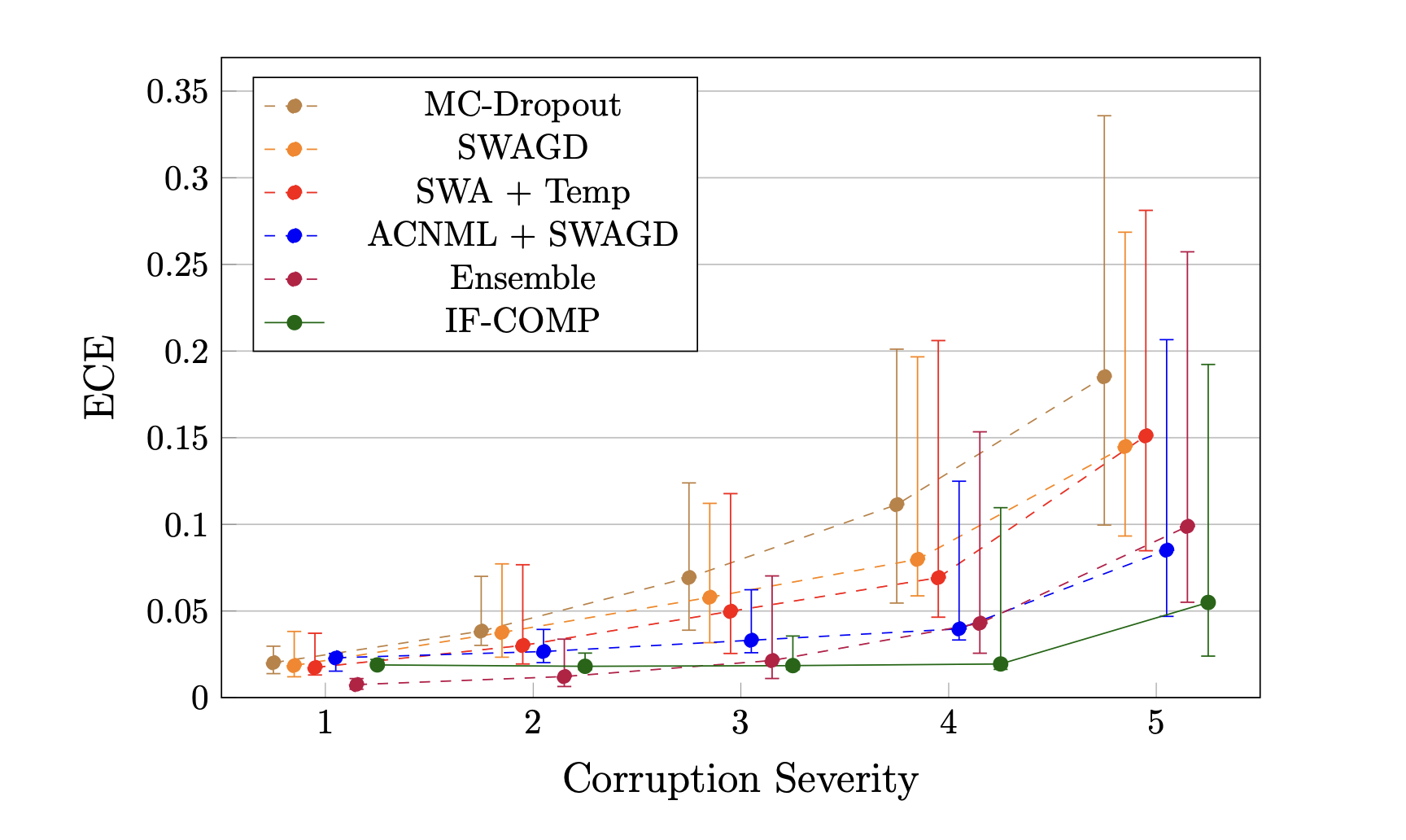Expected calibration error (ECE) for various methods across increasing levels of CIFAR-10C corruptions. We plot medians and inter-quartile ranges.

We find that IF-COMP achieves lower ECE across almost all corruption levels compared to both Bayesian methods and other NML-based methods. We can also tune the specific $\alpha$ value without needing to retrain any models, allowing us to tradeoff between better calibration on low severity corruptions (smaller $\alpha$) and better calibration on higher severity corruptions (larger $\alpha$).

Mislabel Detection: Measuring Complexity on Labelled Data

Can we use IF-COMP to find mislabelled training examples? If an example is mislabelled then we expect a different label to be more compatible, increasing the stochastic complexity. We investigate this hypothesis on CIFAR-10 and CIFAR-100 datasets corrupted with different types of label noise, and measure the AUROC of detecting mislabelled examples.

Mislabel detection AUROC for CIFAR-10 and CIFAR-100 with various types and rates of label noise (best method bolded).

On CIFAR-10 we find that IF-COMP achieves strong detection across all noise types without requiring extra checkpoints, even on the difficult data-dependent noise that other methods fail to perform better than random on. On CIFAR-100, IF-COMP achieves strong performance on symmetric and asymmetric noise, although it fails to detect mislabelled data with human and data-dependent noise, similar to other methods.

OOD Detection: Measuring Complexity on Unlabelled Data

Can we use IF-COMP to detect out-of-distribution (OOD) examples? OOD examples should contain more “essential information” and have many possible compatible labels compared to in-distribution (ID) examples. We investigate this hypothesis on MNIST, CIFAR-10, and CIFAR-100 datasets from the OpenOOD benchmark, measuring the AUROC of detecting OOD examples.

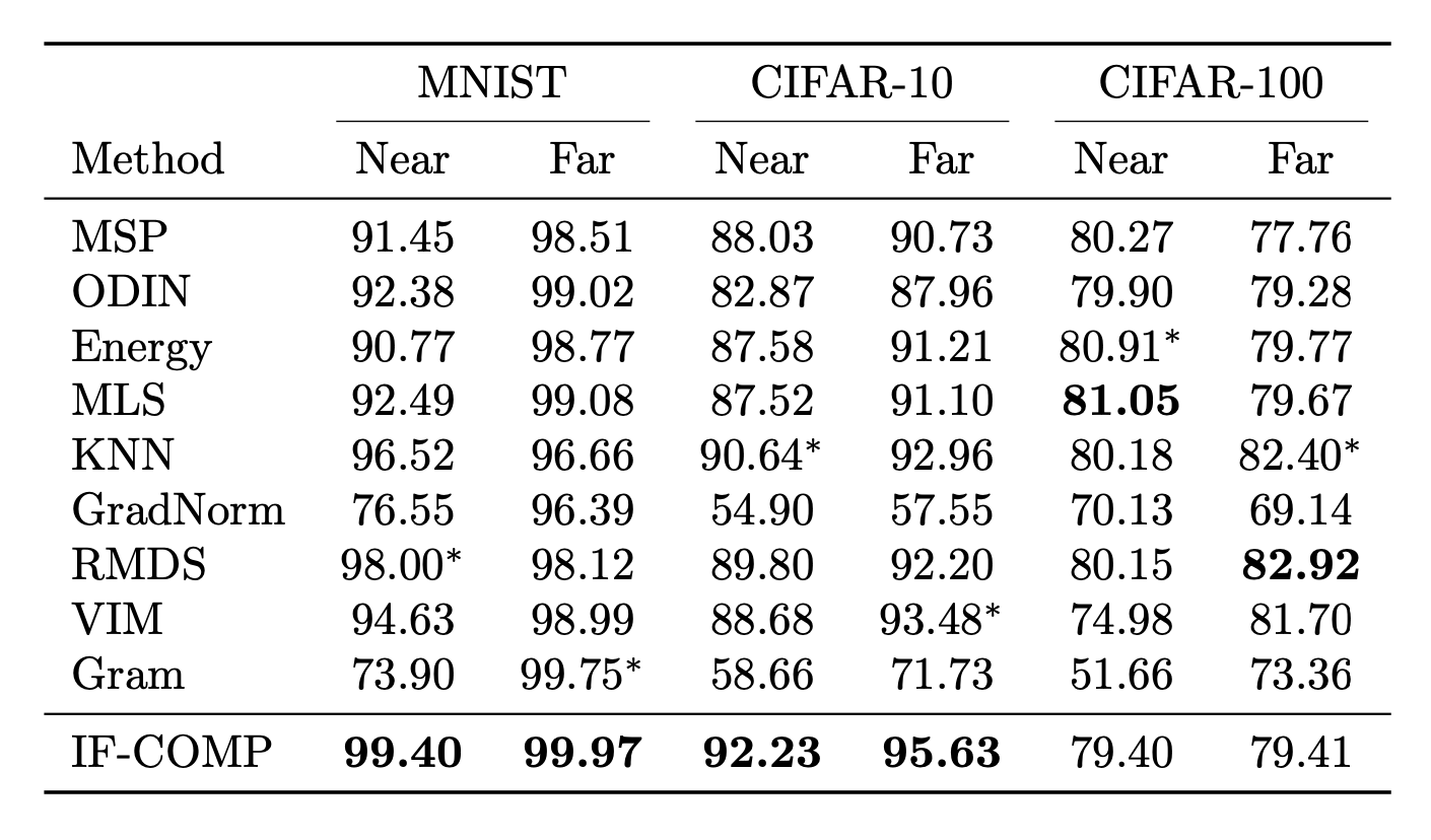
AUROC for OOD detection methods on near and far distribution shifts. Best methods are bolded, and second best methods are starred.

IF-COMP performs surprisingly well on MNIST and CIFAR-10 achieving a new state-of-the-art AUROC for both near and far OOD detection. On MNIST in particular we achieve near perfect detection. Results on CIFAR-100 are a bit less strong, with IF-COMP performing near the middle of the pack compared to other baseline methods.

Analyzing the Components of IF-COMP

How important are each of the different parts of IF-COMP in achieving these strong results? We do a deep dive on our mislabel detection results to see. First let’s look at how the AUROC changes for log error and parametric complexity throughout training.

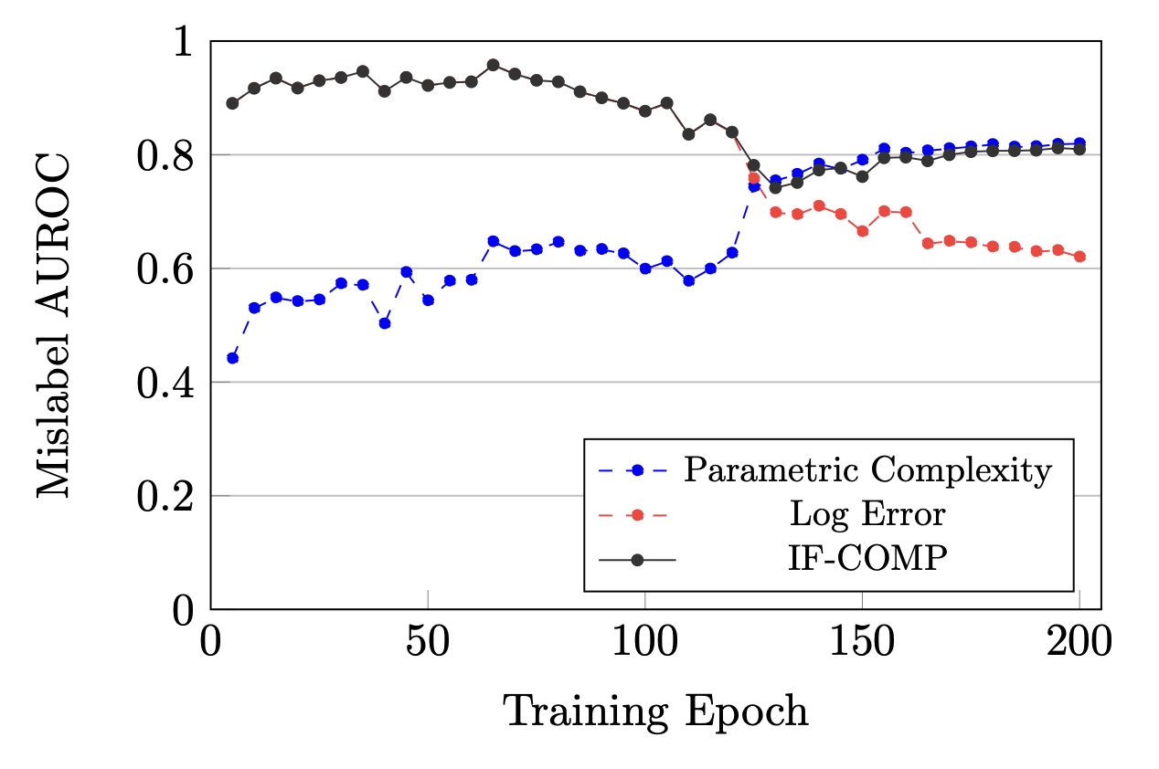
CIFAR-10 mislabel AUROC for each of the individual components of IF-COMP.

We can see that early in training the model ignores the mislabelled data, incurring high error with low complexity compared to correctly labelled data. As we reach convergence, the model learns to memorize this data, lowering the error but increasing the complexity accordingly. The tradeoff between these two values ensures that IF-COMP works at all stages of training both before and after memorization.

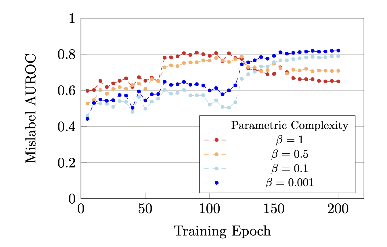
CIFAR-10 mislabel AUROC for the parametric complexity term at varying temperatures.

This tradeoff does not happen without the temperature scaling. At low temperatures the parametric complexity provides no additional signal and mirrors the log error. As we increase the temperature (decrease the inverse temperature $\beta$), we observe the parametric complexity begins to accurately reflect the degree to which the model has memorized the mislabelled examples.

Conclusion

MDL methods are (in my opinion) a compelling way to view learning as compression, and vice versa. Although they may be more difficult to practically apply to deep neural networks, I think they provide many interesting insights into how we can understand the information in data and the learning process. Most of all I think alternative perspectives are especially valuable in the current research climate and give us different ways to understand how and why large foundation models work so well.

---